02: QC and html reports
03-QC_reports.RmdInitial QC and summary
Without any further processing, we can create an interactive html report containing basic summary statistics of the methrix object with methrix_report function.
The report can be accessed here
methrix::methrix_report(meth = meth, output_dir = getwd(), prefix = "initial")
In the report, we can check genome-wide and chromosome based statistics on coverage and methylation, in order to identify potential quality issues, for example:
samples with too high or too low genome-wide coverage or on a specific chromosome. In this case, there is also a possibility, that the sample is affected by copy number alterations. Both methylation levels and coverage therefore shows higher variation among cancer samples.
samples with altered beta level distribution.
A “bump” on the beta level density plot at 0.5 indicates the presence of single nucleotide polymorphisms (SNPs) -> see later.
Filtering
Coverage based filtering
To ensure the high quality of our dataset, the sites with very low (untrustworthy methylation level) or high coverage (technical problem) should not be used. We can mask these CpG sites. Please note, that the DSS we were using for Differential Methylation Region (DMR) calling, doesn’t need the removal of the lowly covered sites, because it takes it into account by analysis. However, using a not too restrictive threshold won’t interfere with DMR calling.
meth <- methrix::mask_methrix(meth, low_count = 2, high_quantile = 0.99)
#> -Masking coverage lower than 2
#> -Masked 280737 CpGs due to too low coverage in sample WT_D14_R1.
#> -Masked 174691 CpGs due to too low coverage in sample WT_D14_R2.
#> -Masked 572896 CpGs due to too low coverage in sample WT_D14_R3.
#> -Masked 313891 CpGs due to too low coverage in sample WT_D6_R1.
#> -Masked 194232 CpGs due to too low coverage in sample WT_D6_R2.
#> -Masked 573417 CpGs due to too low coverage in sample WT_D6_R3.
#>
#>
#> -Masking coverage higher than 99 percentile
#> -Masked 242884 CpGs due to too low coverage in sample WT_D14_R1.
#> -Masked 261635 CpGs due to too low coverage in sample WT_D14_R2.
#> -Masked 216559 CpGs due to too low coverage in sample WT_D14_R3.
#> -Masked 229099 CpGs due to too low coverage in sample WT_D6_R1.
#> -Masked 244079 CpGs due to too low coverage in sample WT_D6_R2.
#> -Masked 215091 CpGs due to too low coverage in sample WT_D6_R3.
#> -Finished in:  14.3s elapsed (11.1s cpu)
Later we can remove those sites that are not covered by any of the samples.
meth <- methrix::remove_uncovered(meth)
#> -Removed 254,494 [0.9%] uncovered loci of 28,217,448 sites
#> -Finished in:  2.494s elapsed (1.818s cpu)
We might want to remove the sites that are sparsely covered. The function coverage_filter has multiple options on how to perform this. We can set a threshold on the coverage and use either min_samples (minimum number of samples) or prop_samples (minimum proportion of the samples) to define the minimum size of samples that should excess the threshold for each CpG side. bsseq requires
#meth <- methrix::coverage_filter(m=meth, cov_thr = 5, min_samples = 2)
#or
meth <- methrix::coverage_filter(m=meth, cov_thr = 5, min_samples = 2, group="Day")
#> -Retained 25,092,237 of 27,962,954 sites
#> -Finished in:  3.011s elapsed (2.307s cpu)
SNP filtering
SNPs, mostly the C > T mutations can disrupt methylation calling. Therefore it is essential to remove CpG sites that overlap with common variants, if we have variation in our study population. For example working with human, unpaired data, e.g. treated vs. untreated groups. During filtering, we can select the population of interest and the minimum minor allele frequency (MAF) of the SNPs. SNP filtering is currently implemented for hg19 and hg38 assemblies.
if(!requireNamespace("GenomicScores")) {
BiocManager::install("GenomicScores")
}
library(GenomicScores)
meth <- methrix::remove_snps(m = meth, keep = TRUE)
#> Used SNP database: MafDb.1Kgenomes.phase3.hs37d5.
#> Number of SNPs removed:
#>       chr      N
#>  1:  chr1 247492
#>  2: chr10 161635
#>  3: chr11 148764
#>  4: chr12 148711
#>  5: chr13 100783
#>  6: chr14 100163
#>  7: chr15  92836
#>  8: chr16 107290
#>  9: chr17 108200
#> 10: chr18  85101
#> 11: chr19  92386
#> 12:  chr2 249923
#> 13: chr20  79069
#> 14: chr21  44901
#> 15: chr22  57855
#> 16:  chr3 198998
#> 17:  chr4 195208
#> 18:  chr5 181417
#> 19:  chr6 187639
#> 20:  chr7 181625
#> 21:  chr8 159936
#> 22:  chr9 130068
#> 23:  chrX  68997
#> 24:  chrY   1325
#>       chr      N
#> Sum:
#> [1] 3130322
#> -Finished in:  00:01:10 elapsed (00:01:02 cpu)
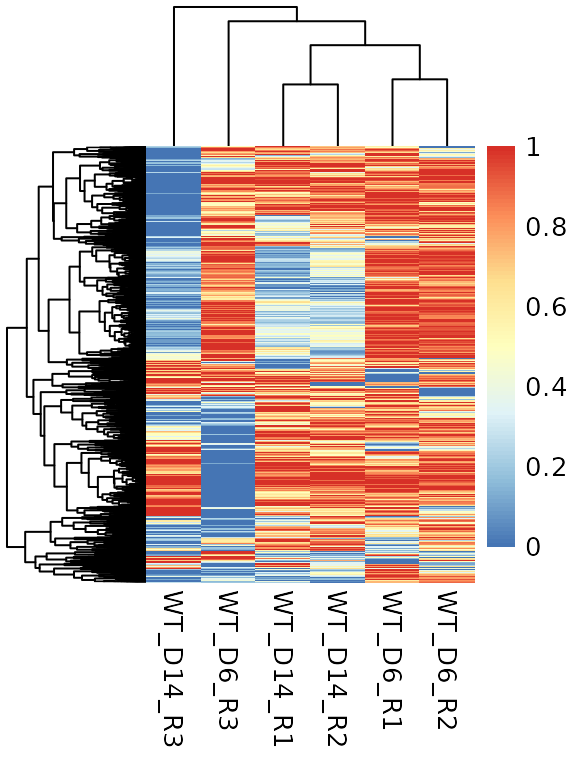
- There is a possibility to keep the sites possibly overlapping with SNPs. We can use this data for detecting possible sample mismatches. For this, we need to plot the most variable sites (probably the ones that are variable in our study population) and plot them on a heatmap.
if (!requireNamespace("pheatmap", quietly = TRUE))
    install.packages("pheatmap")
snps <- meth[[2]]
meth <- meth[[1]]
pheatmap::pheatmap(get_matrix(order_by_sd(snps)[1:min(5000, length(snps)),]))
- SNP removal in mouse data: Usually, there is no need to remove SNPs from mouse data, since for many experiments, the same strain of mice is used. However, there are cases, when different crosses of strains are used, for which, the level of heterozygosity might be different. SNP data for mice can be downloaded from here: https://www.sanger.ac.uk/science/data/mouse-genomes-project. The SNPs can be filtered out using the
region filterfunction.
Visualization and QC after filtering
Methrix report
After filtering, it worth running a report again, to see if any of the samples were so lowly covered that it warrants an action (e.g. removal of the sample)
Important: Don’t forget to set the recal_stats to TRUE, since the object changed since reading in. The output directory has to be different from last time, to avoid using the intermediate files calculated during the last run.
methrix::methrix_report(meth = meth, output_dir = getwd(), recal_stats = TRUE, prefix="processed")
The report can be found here
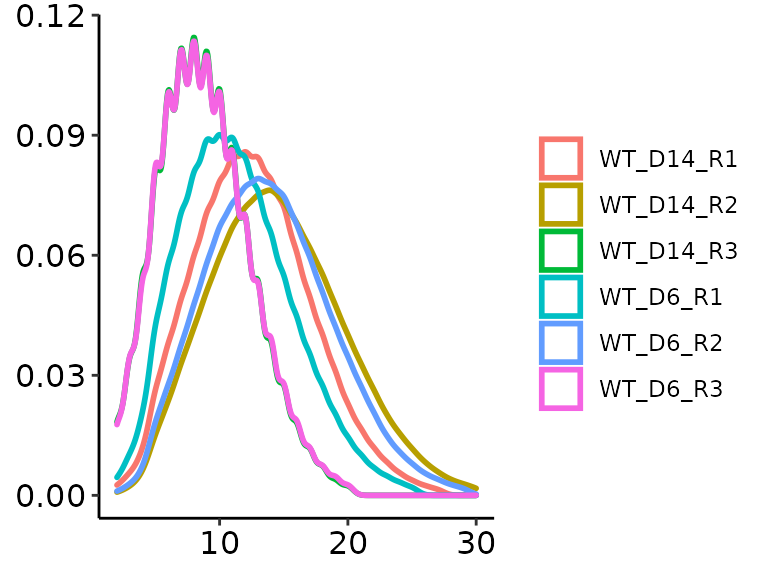
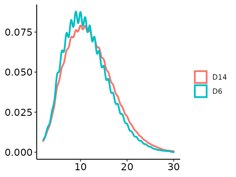
There are additional possibilities to visualize the study. We can look at the density of coverage both sample- and group-wise:
methrix::plot_coverage(m = meth, type = "dens")
methrix::plot_coverage(m = meth, type = "dens", pheno = "Day", perGroup = TRUE)
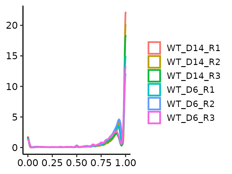
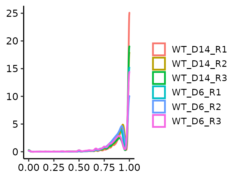
We can visualize te beta value distribution as a violin plot or density plot. These plots (as well as the coverage plot) use the most variable 25000 CpG sites to ensure fast processing. plot_density and plot_violin has the option to use data only from a restricted region.
methrix::plot_density(m=meth)
methrix::plot_density(m=meth, ranges = GRanges("chr22:48007313-49007313"))
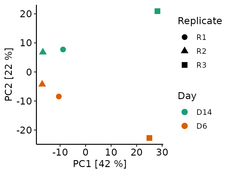
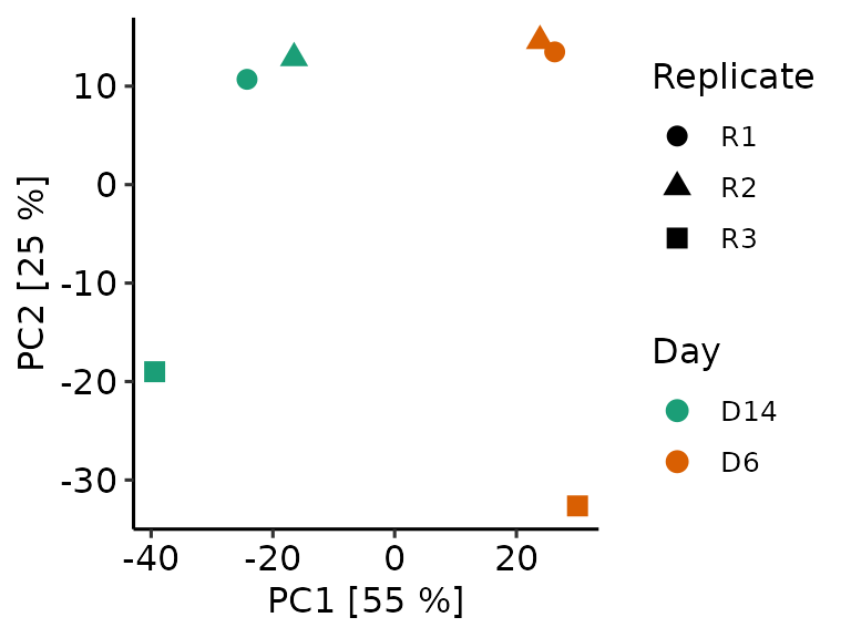
Dimensionality reduction
Methrix offers principal component analysis (PCA) to conduct and visualize dimensionality reduction. As a first step, the PCA model has to be calculated. As for plotting, a given number of sites are selected, either random or based on variance (var option). This ensures that the calculations remain feasible.
mpca <- methrix::methrix_pca(m= meth, top_var = 10000, n_pc = 20)

At visualization, we can provide the methrix object to allow color or shape annotation of groups or samples.
methrix::plot_pca(mpca, m=meth, col_anno = "Day", shape_anno = "Replicate")
methrix offers the possibility of region based filtering. With this option, selected regions, e.g. promoters can be visualized. We will use the annotatr package to assess basic annotation categories.
if(!requireNamespace("annotatr")) {
BiocManager::install("annotatr", update = FALSE)
}
library(annotatr)
promoters = build_annotations(genome = 'hg19', annotations = "hg19_genes_promoters")
promoters
#> GRanges object with 82960 ranges and 5 metadata columns:
#>                 seqnames        ranges strand |             id       tx_id
#>                    <Rle>     <IRanges>  <Rle> |    <character> <character>
#>       [1]           chr1   10874-11873      + |     promoter:1  uc001aaa.3
#>       [2]           chr1   10874-11873      + |     promoter:2  uc010nxq.1
#>       [3]           chr1   10874-11873      + |     promoter:3  uc010nxr.1
#>       [4]           chr1   68091-69090      + |     promoter:4  uc001aal.1
#>       [5]           chr1 320084-321083      + |     promoter:5  uc001aaq.2
#>       ...            ...           ...    ... .            ...         ...
#>   [82956] chrUn_gl000237     2687-3686      - | promoter:82956  uc011mgu.1
#>   [82957] chrUn_gl000241   36876-37875      - | promoter:82957  uc011mgv.2
#>   [82958] chrUn_gl000243   10501-11500      + | promoter:82958  uc011mgw.1
#>   [82959] chrUn_gl000243   12608-13607      + | promoter:82959  uc022brq.1
#>   [82960] chrUn_gl000247     5817-6816      - | promoter:82960  uc022brr.1
#>               gene_id      symbol                 type
#>           <character> <character>          <character>
#>       [1]   100287102     DDX11L1 hg19_genes_promoters
#>       [2]   100287102     DDX11L1 hg19_genes_promoters
#>       [3]   100287102     DDX11L1 hg19_genes_promoters
#>       [4]       79501       OR4F5 hg19_genes_promoters
#>       [5]        <NA>        <NA> hg19_genes_promoters
#>       ...         ...         ...                  ...
#>   [82956]        <NA>        <NA> hg19_genes_promoters
#>   [82957]        <NA>        <NA> hg19_genes_promoters
#>   [82958]        <NA>        <NA> hg19_genes_promoters
#>   [82959]        <NA>        <NA> hg19_genes_promoters
#>   [82960]        <NA>        <NA> hg19_genes_promoters
#>   -------
#>   seqinfo: 93 sequences (1 circular) from hg19 genome
mpca <- methrix::methrix_pca(m= meth, top_var = 10000, ranges = promoters, n_pc = 3, do_plot = F)
methrix::plot_pca(mpca, m=meth, col_anno = "Day", shape_anno = "Replicate")